Fourier Transform Model of Image Formation

What is Fourier transform?

     The Fourier transform belongs to the different classes of Linear transforms.[1] Linear transforms, in essence, "transforms" or "converts" information from one form to another. The Fourier transform, specifically, "transforms" a function with a dimension of G to a function with a dimension of 1/G. Moreover, given this function [say f(x,y)], it's Fourier transform is given by,

Equation 1. Equation for the Fourier transform of an image.

     In this activity, we will be using the Fast Fourier Transform to implement the Fourier Transform. Thankfully, Scilab has functions to implement this. They are fft() and fft2(). In addition, we will be using other Scilab functions that are new to us such as: fftshift(), abs(), conj(), and imcorrcoef().

     We now move on to the tasks we had to do. First off, we had to create a 128 x 128 image of a centered circle with white fill and black background. The image is then opened in Scilab and converted into grayscale.The Fast Fourier Transform for two dimensions was then applied. The intensity values were also computed and the following images were obtained.

Figure 1. (a) White centered circle made in paint. (b) fft2() 

of theimage in (a). (c) fftshift() applied to (b).

     I also did the same procedure for a white circle generated in Scilab. Here is the result:

Figure 2. White Circle generated through Scilab with the 
corresponding outputs of (a) fft2() and (b) fftshift()

     It can be seen that Figures 1 and 2 are almost identical if not for the difference in the radius of the white circle used. In addition to  these, if we apply fft2() again to the output of the fft2() of the grayscale image, we will obtain the white circle itself. Trying a different "object" in the image, we then used the letter "A" as shown below (this was generated through paint for obvious reasons).

Figure 3. (a) Our new "object" in the image. (b) the fft2() 

of a, (c) the fftshift() of (b).

What is a Convolution?

     You can imagine the convolution of two functions to be the smearing of one of the functions to the other. However mathematically, the convolution of two 2-dimensional functions, say, f and g, is said to be given by:

Equation 2. Convolution of two 2-dimensional functions f and g.

     A shorter way of representing the convolution of f and g is through the following manner.

Equation 3. Short-hand notation for 

the convolution of f and g

     Moreover, the convolution theorem states that,

Equation 4. Transform of the convolution h. Note that H, F 

and G are the transforms of h, f and g respectively.

   In this theorem, we see that the transform of the convolution h of two functions f and g is just the product of the transforms of f and g. And in the activity, we were tasked to do the following: (1) Create a 128 x 128 image with the letters VIP in it. I created this image using paint making sure the the letters occupy approximately 50% of the image. The font I used here is Arial. Here is the image,

Figure 4. Our object

     I then created another 128 x 128 image. A centered circle with white fill and black background. This image becomes our "aperture" of a circular lens. The next thing that we should do is to implement fft2() to Figure 5 and to  apply fftshift() to our aperture. Having done these, we multiply the two and get the inverse then display the modulus. Note that I varied the radius of the circle to observe the effect on the resulting image. The resulting images with the corresponding circles are seen in Figure 5.

Figure 5. Imaged "VIP" with corresponding lens aperture. The columns 

give a particular lens aperture with its corresponding imaged "VIP".

     The first observation that came to me when I saw these results (besides the fact that the resulting image is "upside down") is the quality of the resulting images. As one increases the radius of the circle the quality of the resulting image becomes better. Obviously, among all of these (including the object) the object has the greatest quality. 

What is Correlation?

     We now move on to correlation. In a nutshell, the correlation of two functions f and g gives the "extent" or degree of similarity of the said functions. [1] Mathematically, it is expressed as,

Equation 5.  Correlation of the two-dimensional functions f and g

     This can be written conveniently as,

Equation 6. Short-hand notation for the correlation
of two 2-dimensional functions f and g

     In addition, correlation is related to convolution in the following manner,

Equation 7. Relation of correlation to convolution

where the asterisk at f asks for the complex conjugate of f. Also, the transform of the correlation p is given by,

Equation 8. Transform P of the correlation p.  F and G are the transforms 

of  f and g respectively. F* is the complex conjugate of F

     Since the correlation gives us the degree of similarity of two functions, it is often used   in Template Matching. Template Matching is a technique used to detect parts of an image that match a particular template. [2] In the activity, we used an image with text to apply this technique. A template of a letter included in the text was then created. Note that the same font and font size for both the text in the image and the template was used. The results are shown below.

Figure 6. Application of correlation in an image with text. 

(a) template, (b) image with text. (c) resulting image.

     In Figure 6c we see the result. Note the positions of the letter "A" in (6b). If we compare it with Figure 6c, we see something interesting. Upon getting the transforms of (6a) and (6b) and applying it to Eq. (8) we get the transform P. And, taking it's inverse transform allows us to know the correlation p. Since the correlation gives us the degree of similarity between the template and the text in the image we know that the "brightest points" in (6c) has a high degree of similarity and therefore these letters match our template which is confirmed through our result. 

     

     Another thing that we did for correlation is edge detection. We used different patterns which were basically 3 X 3 matrices. The sum of all the elements in this matrix must be equal to zero. We then convolve this pattern with Figure 4. The result for each matrix is seen in Figure 7.

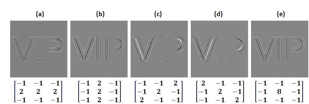
Figure 7. Results for edge detection using different patterns of edges. 

(a)  horizontal pattern, (b) vertical pattern, (c) diagonal pattern going 

from left to right, (d) diagonal pattern going right to left,  and (e) spot

pattern.

     That ends our activity (Fourier Transform Model of Image Formation). It took me quite a long time to finish. However, I'm really amazed that I have finally finished it. Honestly, it's not that hard. It's actually quite simple and fun! And for that, i'd give myself a grade of 7 out of 10. All the images are of good quality and are with understandable captions. The 3 point deduction is due to the fact that I was late in posting my blog for this activity. Nevertheless, I had fun with this activity

     Thanks to Jen-Jen Manuel. Her post on this activity helped clarify some confusions with some of my results. 

All glory to God!

References:

[1] Soriano, M. A6 – Fourier Transform Model of Image Formation. Applied Physics 186 Manual. 2010.

[2] Template matching, retrieved September 22, 2011, http://en.wikipedia.org/wiki/Template_matching 

Raw Egg and Adobong Pusit

Sometimes what we see can be deceiving. When this happens there are instances that our discernment fails and we become deceived. As an example let me tell you a story. During my pre-school to early elementary days the only food i'd eat when I didn't like the food served in our house is raw egg with rice. Yes, RAW EGG!  During meal times I'd ask for a bowl, an uncooked egg, some salt and rice then mix them all together. I remember eating this odd combination for a long period of time (say a few years. HAHA.). I'd happily eat it because, to me then, the other food that the people around me were trying to feed me didn't look delicious. A few years into this raw-egg-with-rice phase of mine I was slowly losing the desire to eat raw egg and I became more and more interested to taste other food. The combination seemed to taste more and more bland. And it finally dawned on me, "What i'm doing is disgusting and it tastes horrible!" (Sorry if I offended any raw egg lovers! :D) I could only remember one of the Sundays where I actually tried to eat something different. It was during a family lunch in my grandmother's house. I dared to eat Adobong Pusit (Squid). I remembered it tasting really good. I didn't know it at that time, but, now that I look back it was a turning point in my life. When I decided to ignore the appearance of what I was about to eat and instead focus on what it was going to taste like. I was going to free myself from years of slavery to the raw egg. For years I had been boxed, never tasting other food only because I considered the appearance more than the taste. I had missed out on the real and good stuff! "Chill Haneka! It's just food." Yeah, it is. But, in our lives we can be like this sometimes. We are boxed because we consider what we see to be more important than what that person/situation/thing really is. We miss out and fail to enjoy.

Yummy! HAHA.

In this activity, we are trying to enhance images in order to see the information captured by the recording instrument. And just like my raw egg dilemma, hopefully we'll be successful to "see" beyond the limitations of what we can see. 

First off, I picked a dark colored image so that I can do some enhancing to it. The said image can be seen below.

Truecolor Image
Source:  http://www.designzzz.com/gorgeous-sunrise-photography/

I then converted the image to a Grayscale image using the gray_imread function in Scilab. The resultant image is shown:

Grayscale Image

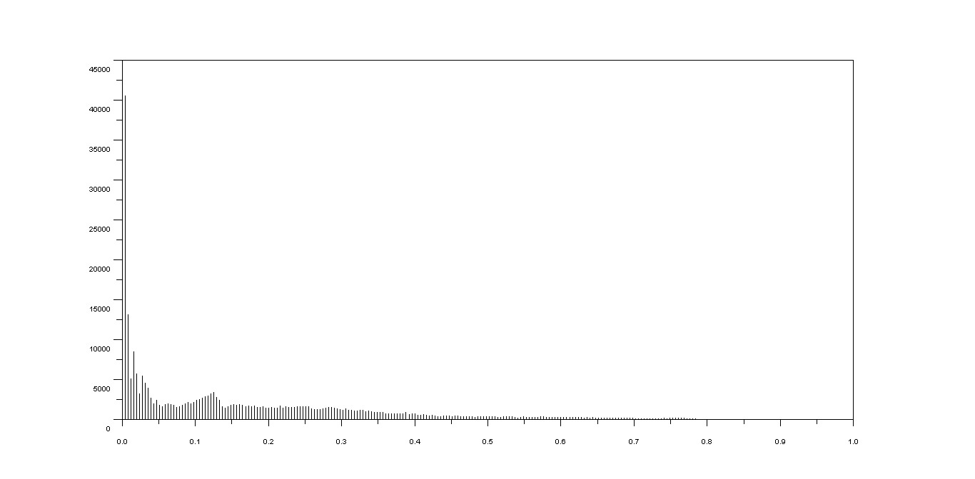
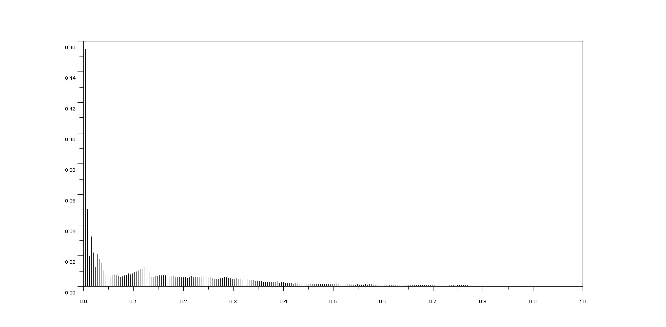
Having this image, I got it's histogram using my own code then normalized the histogram to create the Probability Distribution Function (PDF) of the image. The PDF of the image gives us an idea of the probability of a certain gray level to be present in the image. The code, histogram, and PDF can be seen below,

Histogram Code. Pixel Frequency versus Gray level values.

Histogram of the image. the x-axis is the gray level while the y-axis is the
pixel frequency.

Code for the PDF or normalized Histogram of the image.

PDF of the image. x-axis is the gray level while the y-axis is the percentage of pixels.

Moving on, here comes the part where our brain muscles will need a slight programming work out. Breathe in. Breath out. To enhance the image we can manipulate the histogram of the grayscale image. We will be able to do this by creating a desired Cumulative Distribution Function (CDF) for the resulting image. We will then back project the grayscale values using the  CDF in order to modify the PDF of the image. Now that we know that, let's first create the CDF of our image. Using the function cumsum we can easily do this. Both the code and plot can be see below:

Cumulative Distribution Function code

Cumulative Distribution Function plot of the image

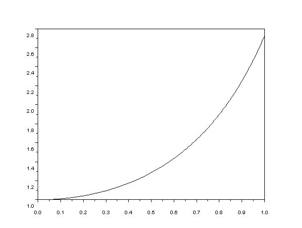
Now that we have the CDF, we will create our desired CDF for the enhanced image. I have created to such CDFs. One is linear and the other one is exponential. The CDFs and corresponding codes are given,

Code for Desired CDF (linear)

Desired CDF (linear)

Code for desired CDF (exponential)

Desired CDF (exponential)

We're one step closer to enhancing our image. The next step would be to backproject. Thanks to a great function in Scilab called interp1, we can easily do this. 

Code for backprojecting using a desired CDF that is linear

Code for backprojecting using a desired CDF that is exponential

The next thing to do is to finally apply the changes made to enhance the image. Unfortunately I wasn't able to  finish this part(I wasn't able to figure it out on time :( ).

Other than image enhancement using Scilab, we also got to play around with Gimp. Here I loaded the same image and once again converted it to a grayscale image. After this, I was able to play around with the image using one of the "tools" in Gimp  called curved which can be found in the Colors section of the menu. Below are the images I played with (From simple grayscale to totally odd effects.)

Effects of image manipulation in Gimp

Curve "tool" in Gimp

Curve tool in Gimp

Effects of image manipulation in Gimp

Curve tool in Gimp

Curve tool in Gimp

For my self-evaluation,  i'd give myself a 7 out of 10 since I wasn't able to finish it. Special thanks to Jen-Jen Manuel, Elo Anguluan, Tracy Estella, Kirby Cheng, and Dr. Soriano :)

God bless everyone! :D

Uncertain No More :)

NOTE: There are people who might not agree with the contents of this blog. However, I challenge you (yes you!) to read on and read on to the very end!

Estimate: (verb)

1. To calculate approximately (the amount, extent, magnitude, position, or value of something).
2. To form an opinion about.

There are points in our life where we find ourselves estimating. Depending on the context, sometimes we estimate the time we would take to prepare for work or for school. There are times we estimate the money we'll be spending to pay for our bills. Sometimes, we even estimate people. To be honest, now that I think about it, I personally don't like estimating. Why, because sometimes whether we like it or not, estimates are not accurate. When that happens we become disappointed and that is hard to take in. But me not liking estimates does not remove the fact that I do estimate.

Let's look at estimates in the context of our personal lives. Doesn't it bother you that there are things in your life wherein which you can't be sure of? Doesn't it? Think about it. We are not sure of many things in life. Yes, we can estimate but nevertheless we are not sure. You might say, "Haneka, that's the thrill in life! We get surprises every day." I don't disagree with that. Life would be boring if we knew what would happen to us every single day. But, if I may ask, what if there is a way to be sure? 

In Quantum Mechanics, we are taught the Uncertainty Principle. Simply put, this principle says that two quantities (say, present position and future momentum) cannot be simultaneously measured with high precision. This means that one quantity can be measured precisely; however, the precision of the other quantity to be measured will be compromised. The more you run after one to obtain an answer the more you lose the other. In life, there are things that we just can't be uncertain of. There are things that we just can't estimate. There are times where in we are demanded to decide - yes or no. We can't afford to be in the gray area. It's either we're hot or we're cold.

Now that we have considered this, let us ask again: What if there is a way to be sure of things? What if there is something or, better yet, someone that can help us know. In the bible, it says that:

^"6Jesus said to him, 'I am the way, and the truth, and the life. No one comes to the Father except through me.' "

John 14:6(ESV)

In this verse we find Jesus, saying that He is the truth and that He is the life. You see, until we know the Truth we are deceived by lies and we become blind. And, until we know the Life we have no life. And as long as we continually try to save ourselves and be lord over our own lives, we'll lose our life. "So Haneka,", you might ask, "what does all this have to do with estimation?" You see, if there is one thing that we can't estimate, it's where  we'll go when we die. We can't just estimate that and find out at the end that we're wrong. This might be too heavy for some of you, but I'd rather let you people know it now. 

In Jesus there are no estimations. In Romans 10:9 it says that:

⁹ If you declare with your mouth, “Jesus is Lord,” and believe in your heart that God raised him from the dead, you will be saved. 

Romans 10:9(NIV)

Wow! We finally have a way and right to be certain - no more estimation. We don’t have to estimate whether we have done enough good works to earn ourselves a spot in heaven. We don’t have to worry ourselves to death on whether we’ve believed in Him enough for Him to spare us the pain of hell. Why, because the job is already done. Our sins have been paid at a price (Yes, you’re a sinner and so am I.) Don't get me wrong, there are things that we do have to trust Him for - things in our life that we still do not see. But God will never forsake us. And the one thing that we cannot be uncertain of, he made certain for us already.

It’s likely that some, or majority, of the people reading this blog know me as Haneka, an Applied Physics student, their batchmate, their classmate, their labmate and their friend. You might be thinking, “Haneka, you have no right to tell me what to believe in.” To a certain extent, you have a point. I have failed more subjects than the average student. I am challenged by the subjects I am currently taking. I fail and disappoint myself and others at times. And I too am uncertain of different things. But despite my imperfections, there is one thing that gives me the boldness to speak to you. And of this I am certain: That my God loves me. and  He has bought me at a price - His life. That, to me, is the only thing that really matters.

Moving on to the part of my blog where I am actually being graded. :D

Our activity today dealt with area estimation using images. To help us warm up, we had to create a black and white image of a regular geometric shape using paint or Scilab. The actual area of the shape that we will construct must be known. Using Green’s theorem, we were to calculate the area enclosed by the shape. I chose to make a square using Scilab. I utilized one of the methods I previously used in our second activity (link here). Here is the image I produced:

Figure 1. Square with white fill and black

background generated using Scilab.

It is important to make sure that the image of the square has a white fill, black background, and is saved as a BMP file. One of the reasons is because we will be using a built-in function in Scilab wherein objects must be binary. I then load this image into my Scilab console and implement the function follow. This function, in essence, gets the parametric contours of the object [x(i), y(i)]. We can then use the obtained x and y values, in implementing Green’s Theorem. Results are shown in the table below:

Table 1.Actual area and estimated area

using Green’s Theorem

Before we proceed, I want you guys to see the discrete form of Green’s theorem,

Green’s Theorem (Discrete Form)

Also, here is the code I used to implement Green’s theorem,

Figure 2. Green’s Theorem code for Square area estimation

Note that there was a problem with my SciPad when I tried to execute the code. Hence, I had to resort to entering the code line by line in the console.

After the “warm-up”, we had to pick a place, through Google Maps. We will use the image to estimate the area of the place. I picked the newly built CS Amphitheater. Here is the “raw” image.

CS Amphitheater in the National Science Complex of the Univeristy

of the Philippines as seen in Google Maps

To calculate the area using the same concept we must first think of a way to convert this image into a binary one. What I did was to overlay a circle (white fill) on the image where the circular outline of the amphitheater is. I then used a square shape to underneath the circle to cover the other parts of the image. However, when I checked the image type in Scilab, it was still a true color image. So I converted it to a binary one using the function im2bw. Here is the binary image:

Binary image of the edited CS Amphitheater image

I then implemented the following Green’s theorem through the following code: 

 Green's Theorem for CS Amphitheater area estimation

I then obtained the following results:

Table 2. Results for CS Amphitheater area estimation

Also, assuming that the amphitheater is a circle, I measured its radius using a tool in Google Maps. It turns out to be: 36.6883 m. Therefore, the total area occupied by the amphitheater is: 4228.682 m².Our next concern is to convert the results we got from Scilab to actual meter values. We can do this by using the scale in Google Maps (as seen in the lower left corner of the raw image), and through the method introduced in activity 1, convert the pixel values into actual meter values. I was able to obtain a best fit equation of y = 0.289x – 10.14. However, when I plugged in the Green’s theorem the result for the area was a surprising 15,645.9 m². This has a 72.97251 % error when compared to the actual meter values. This is perhaps due to an error in the code or in the manner of obtaining the best fit equation. Therefore, for this activity, I’d give myself 9 out of 10 since I was able to understand the topic and captions can be understood. The 1 point deduction is due to the large percent error.

Note: My sources are the links I used. :)

I would like to thank Jen-Jen Manuel, Kirby Cheng, Dr. Anthony Longjas for all the technical help they gave. Also, thanks to Lory Manalo for “proof reading”. Hannah Olid, you know what I’m thanking you for. And of course, to my God who has sustained me at all times, thank You and I love You.