A9 – Morphological Operations

     According to the thefreedictionary.com morphology is the form and structure of anything. And,  perhaps in this post we will not be dealing with "anything" but nevertheless we will be dealing with  form and structure. To start off, let me introduce four (4) shapes that we will be working with: (1) a 5 x 5 square, (2)  a triangle with 4 boxes as base and 3 boxes as height, (3) a 10 x 10 hollow square whose walls are 2 boxes thick, and lastly (4) a cross that's 1 box thick and 5 boxes along the horizontal and vertical.

Figure 1. Objects(1) a 5 x 5 square, (2)  a triangle
with 4 boxes as base and 3 boxes as height, (3) a
10 x 10 hollow square whose walls are 2 boxes thick,
and lastly (4) a cross that's 1 box thick and 5 boxes
along the horizontal and vertical.

     Now let us look at the structuring elements or SE

Figure 2.Structuring Elements (SE)

     Given the 5 different structuring elements, our task is to perform erosion and dilation in each individual object. Therefore, starting with erosion:

  

   We now move on to dilation,

     Lastly, the function thin in Scilab outputs the "internal skeleton" or a thinner version of the input. Also, the function skel acts in a similar manner.

In this activity, I will give myself a grade of 8 out of 10.

Thanks goes to Eloise Anguluan. Her step by step post on how to erode and dilate helped me a lot. Thanks also to Jen-Jen's post.

God bless everyone!

References:

1 Soriano, M. Morphological Operations. 2010. Applied Physics 186 Activity Manual

A14 – Color Image Segmentation

There are instances where we need to extract information from only a certain portion of an image. When this happens, we find ways to eliminate other unnecessary information in the image so that we are left with what we want. In this blog, I will be discussing two techniques in Color Image Segmentation. 

Shown in Figure 1 is the image we want to segment. Here, our region of interest or ROI is the the apple (minus the leaf). Later on, we can choose another region to be our ROI.

Figure 1. An image of an apple. This is the image
where we will apply Color Image Segmentation.

I. Parametric Segmentation

For this method, we need to crop a portion of our region of interest in the image. For this case, I cropped a portion of the apple. This is shown in Figure 2.

Figure 2. Cropped portion of our
ROI in Figure 1.

Note that the image I used is a True Color Image. This is crucial since we need the RGB values in this method. Given the Figure 2's RGB values, we are to use them in "expressing" the Normalized Chromaticity Coordinates (NCC) which is shown in Eq. (1).

Equation 1. Normalized Chromaticity Coordinates (NCC). R, G, and B are the respective
RGB values of the image per pixel, while I is the sum of these values per pixel.

Upon converting the RGB values into the NCC we can now obtain the joint probability p(r)p(g). Where p(r) is given by,

Equation 2. The probability that a pixel with chromaticity
r belongs to our region of interest.

To obtain p(g), simply replace all instances of r in Equation 2 with g. Upon execution we see the resulting segmented image.

Figure 3. Segmented image using Parametric
 Segmentation

Let us now try using the leaf as our ROI. Using the corresponding portion:

Figure 4. Cropped portion
of our new ROI.

we obtain the following segmented image,

Figure 5. Segmented image using
Parametric Segmentation.

II. Non-Parametric Segmentation

In non-parametric segmentation, we need to take the 2D Histogram of the corresponding r and g values of a portion of our ROI. Let us consider the following histograms,

Figure 6. (a) Normalized chromaticity space (b) 2D Histogram 

. . . . . Although I didn't finish this work, I still give myself an 8 out of 10.

Thanks to Dr. Anthony Longjas.

God bless everyone!

A8 – Enhancement in the Frequency Domain

     If you haven't noticed, there have been previous posts here in my blog regarding Fourier Transforms, it's properties and the like. This is because knowing these tools (if you may) can help us in achieving "bigger" things. That having been said, in this activity we will utilize what we know so far of the fourier space and apply it to different situations. 

PART A: CONVOLUTION THEOREM

First off, let us look at the following 2D patterns:

Figure 1. (a) Two dots lying on the x-axis and symmetric about the y-axis.
(b) The modulus of the Fourier Transform of (a).

Figure 2. The first row is composed of images of two circles
of varying radius lying on the x-axis and symmetric about the
y-axis. The second row is the modulus of the Fourier Transform
of a respective pair of circles. 

      We have already seen Figure 1 in a previous blog. Now, instead of dots let us use circles of varying radius. From Figure 2, we observe that the FT modulus of our 2D pattern is given by "distorted" concentric circles. Moreover, as the radius of the circles increase the size of this interference pattern decreases. 

Figure 3.The first row is composed of images of two squares
of varying side length lying on the x-axis and symmetric about the
y-axis. The second row is the modulus of the Fourier Transform of a respective pair of squares.  

     What if we replace the dots with squares instead of circles? In Figure 3, we see exactly that. In addition, given the respective fourier transform of each pair of squares we see that as the side length increases the  width of the distorted cross or plus sign  (interference pattern) decreases. 

Figure 4. The first row is composed of images of gaussians
of varying variance. The second row is the modulus of the
Fourier Transform of a respective gaussian pair. 

     Let us now try another 2D pattern - gaussians of varying variance. As seen in the Figure above (Figure 4), the interference pattern size decreases as the variance decreases. This trend is similar to the first two patterns.

     Another interesting thing that we will look at now is the convolution of two images. In Figure 5b we see the the result of the convolution of a vertical line (3x3) with the set of random points shown in 5a. What we see in 5b is the replication of the vertical line in every location where there is a random point. 

Figure 5. Convolution. (a) Random points. (b) Convolution
of a vertical line (3X3) to the random points of (a).

     To end this section, let us look at Figure 6. Our pattern are images with equally spaced dots that are on the x and y axis. Their corresponding FT modulus are also given in the figure.

Figure 6. The first column is composed of images of equally
Spaced dots lying on the x and y axis. The second row
is composed of the modulus of the FT of the images in the
first row. 

PART B: FINGERPRINTS: RIDGE ENHANCEMENT

Figure 7. Fingerprint (source)

     Given an image of a fingerprint, we can enhance the identifying marks or ridges in that fingerprint by masking unwanted frequency in the fourier  domain. We start with the following:

a. Take the Fourier transform of the image.

b. Design a filter for it.

c. Apply filter.

Figure 8. (a) FT modulus of Figure 7, (b) the filter I chose
to mask unwanted frequencies, and (c) Resulting image.

     Note that the output is not quite right. I would have to say that the error came from the choice of mask used.

PART C. LUNAR LANDING SCANNED PICTURES: LINE REMOVAL

     Applying masks can also be used in removing unwanted portions of an image. Here, we have an image where unwanted vertical marks is to be removed. I used the following mask in "filtering" the image.

Figure 9. Filter used in the image.

     Upon applying this, I was able to obtain the image in Figure 10b. I would have to say it looks pretty good.

Figure 10. (a) Image with unwanted vertical lines, (b) filtered image

PART D. CANVAS WEAVE MODELING AND REMOVAL

     Here is a similar case to the previous section. However, in this case we need to remove the weave marks instead of vertical lines. Shown in Figure 11 is 

Figure 11. Filter choice

Figure 12. (a) Image with weave marks. (b) filtered image.

     Unfortunately, it looks like the marks weren't removed. Once again, I strongly believe the error is in the choice of the filter.

Figure 13. (a) Inverted Filter. (b) FT modulus of (a) 

     Lastly, inverting the filter and taking it's FT modulus, we try to compare it with the weave pattern. Unfortunately, it does not resemble the weave pattern. However in my opinion it reminds me of the pattern (in an artistic manner) :D

     For this activity, I give myself a grade of 8 out of 10

     

     I'd like to thank the following people for their blogs: Jen Jen Manuel, Krista Nambatac, Tisza Trono, and James Pang. Because of their posts I am able to check my work and better understand the activity.

     God bless eveyone! :)

A12 – Preprocessing Text

Given a scanned image of a document containing handwritten or printed elements, one can actually apply image processing techniques to extract these desired elements. Specifically, documents with almost unrecognizable letters or words can be processed to make them understandable. In this blog I will be discussing some of the techniques I used in order to process one specific document with both handwritten and printed elements.

Figure 1. Scanned image of a document with handwritten and
printed elements.

Shown in Figure 1 is a demonstration equipment receipt or a demo checklist. I applied image processing techniques to a portion of this document. I started out by selecting an area where both handwritten and printed texts are present. Knowing that the image is tilted, I then used the Fourier Transform of the image to determine its tilt angle. Using some help from Adobe Photoshop CS 3 we can get the difference between the angle made by the vertical axis with respect to the horizontal axis and the angle made by the Fourier Transform with respect to the horizontal axis as well. Figure 2 can help clarify this.

Figure 2. (a) An enhanced image of the Fourier Transform of Figure 2.
(b) The tilt angle of the image.

Using this method, the tilt angle of the image was found to be 1.3 degrees. To "correct" this, we used the Scilab function mogrify. Upon executing this, we obtained the following result:

Figure 3. (a) Grayscale image of the document portion (Note that the tilt is
 not yet corrected.).  (b) " Corrected" image.

Now that we have corrected the tilt, the next thing that we are going to do is to remove the horizontal lines in. In doing this, we are able to isolate the words, thus, helping us understand what is written.

A15 - Pattern Recognition

    In image processing, a pattern is a set of features. [1] These features can be the color, size, area, or shape of an object. Depending on the value of these features we can classify our objects. If a group of objects have more or less the same features, then they belong to the same class. 

    Look at it this way, features make up the signature of a specific object. Note that, no matter how legibly a person writes, no matter how hard that person tries to recreate an identical copy of one of his signatures, he will fail. There will always be a difference each time he/she signs. However, this doesn't remove the fact that that signature belongs to that particular person. Same goes with object features. Objects may not be completely identical, but to a degree they are such that they can be classified under one group.

    In this blog, we will be classifying objects based on their features. This type of task is commonly called Pattern Recognition. Some applications of pattern recognition are: 

1. the automatic recognition of handwritten postal codes on postal envelopes and [2] 
2. the automatic recognition of images of human faces. [2]

Figure 1. Face Recognition.
Click to go to source.

Figure 2. Handwritten Letter.
Click to go to source.

 For this activity, we will be looking into 4 classes and extract features from them. The first feature will be area. 

References

1. Soriano, M. A14 - Pattern Recognition. Applied Physics 186 Activity Manual. 2008.
2. Pattern Recognition, Retrieved September 20, 2011, http://en.wikipedia.org/wiki/Pattern_recognition

Properties of the 2D Fourier Transform

     In one of my previous blog posts, I have "introduced" the Fourier Transform. And now In this blog, we will be looking at its properties. This is important, because if we know some of its basic properties we will be able to, somehow, understand more complex situations involving Fourier Transforms.

     Below are some 2D patterns and their respective Fourier Transforms. I obtained the Fourier Transforms using Scilab.

Figure 1. 2D patterns with their respective Fourier Transform. 

A column corresponds for  a 2D Pattern - Fourier Transform 

pair. (a) Square, (b) Annulus, (c) Square Annulus, (d) Two slits 

along the x-axis and (e) 2 dots symmetric about the center.

     In  Figure 1 we see that given a certain 2D pattern, we obtain a distinct Fourier Transform. Note that in this particular work, the two slits  (Figure 1d) are symmetric about the center. Keeping these patterns in mind are important if we want to know more about Fourier Transforms. Moving on, below are 2D sinusoids along the x-direction. Just like in the first set of patterns, I took their Fourier Transforms. And as we see in Figure 2, as the frequency of the sinusoid increases, the distance between the two dots in the transforms of the sinusoids increases.

Figure 2. 2D sinusoids with their corresponding Fourier Transform.
A column represents a sinusoid-FT pair. (a) f =  4, (b) f =  8,
(c) f =  12, and (d) f =  16.

    Since digital images have no negative values, we add a bias to the sinusoid. Just like this,

Equarion 1. Sinusoid with bias A.

     Here A is the bias. And upon execution, we have the following:

Figure 3. Sinusoids with bias. (a) Constant 
bias of 10 and sinusoid frequency = 8, and (b) 
Sinusoidal bias of frequency 0.5 with same f = 8.

     Notice that in comparison to Figure 2b the FT of sinusoids with a bias has additional points. Specifically, for the constant bias, a dot at the center of the image can be seen, while two faint dots at the upper and lower portion of the images are present.  Given a non constant bias, two dots appear symettrical about the center in line with the y-axis. All of these dots (from the constant to non constant bias) obiously represent the FT for the respective biases.

     Let us now try to experiment with our 2D sinusoid. What if we rotate it? As seen in Figure 4 rotating the sinusoid also rotates its Fourier Transform. Once again, this fact is very helpful. Let us keep this in mind.

Figure 4. Rotated Sinusoids with respective Fourier Transforms.
(a) theta = 30 ,  (b) theta = 60, (c) theta = 90, (d) theta = 120

     We now go to combinations of sinusoids. By combinations I mean product of sinusoids. And below, we see just that. Note that the observation that as the frequency of the sinusoid increases, the distance between the two dots also increase is also evident in Figure 5.

   

Figure 5. Combination of sinusoids in the X and Y together
with their respective Fourier Transforms. (a)  f =  4 , (b) f = 8.

Lastly, below are combinations of "regular" sinusoids and rotated sinusoids.

Figure 6 Combinations of "regular" sinusoids and rotated
sinusoids. (a) X-Y-Rotated, (b)  X-Rotated, (c) Y-Rotated

For this activity, I would give myself a grade of 9 out of 10. 


I would like to acknowledge Jen-Jen Manuel and James Pang for their blogs. It helped me better understand this activity :)


God bless everyone! :D

Basic Video Processing

     In this present day and age we are blessed to have new technology that help us in our daily lives. Such technology is the Video technology. Videos have been around for quite some time and its uses have evolved over the years. As a matter of fact, for the children of today, a video is something common. We sometimes forget that people in the past didn't have the same technology that we have. Back then, the "videos" that people knew were different from the "videos" that we now know. For example, in Figure 1 we see a Zoetrope, a device that consists of a hollow drum with pictures positioned at the bottom third of the drum. These pictures make-up a sequence of events. These pictures can be viewed via slits on the drum. The drum is mounted on a spindle such that one may be able to spin the drum. Upon spinning, one can see the pictures as if they were "moving". [1] 

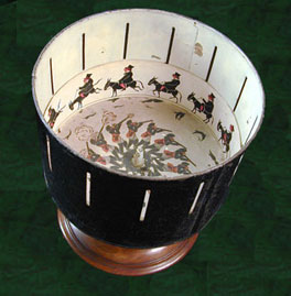
Figure 1. A Zoetrope [1]

     The videos of today may seem far from what "videos" were before, however the essential concept is preserved. Videos are made up of images constituting a sequence of events. They're applications or uses may be different but the main concept remains relatively unchanged.

     Also, images of successive events are very useful in gathering details regarding those specific events since it gives us an idea of the time element involved. This is contrary to a single image which only gives us information at a single point in time. Using image processing techniques we can extract information in a particular situation even without actually being there. Therefore, as an example, I will be discussing the Physics behind a free falling ball captured on video - an experiment me and my partner Rusty Lopez did for this post.

First off, the materials we used are the following

• Sony Cyber-Shot W310 Camera (Thanks to Eloise Anguluan)
• An orange ball (Thanks to Eloise Anguluan again)
• A metal ruler (Thank you IPL)
• Scilab (our image processing tool)
• Stoik Video Converter
• VirtualDub

     We recorded our video using a Sony Cyber-Shot W310 camera. We then used Stoik Video converter to change some of the details in our video such as frame size and frame rate. We also compressed the video into black and white and "muted" out the sound. The output format of our converted video is in AVI for PC small. After doing this, we marked or cropped out the important segment of the video using VirtualDub. Make sure to save the "cropped" version as an AVI file. We then loaded the cropped version of the video into VirtualDub with the intention of "segmenting" it into frames. This can be done by clicking "File" then choosing "Export" and finally selecting "Save as Image Sequence". The resulting frames are shown below.

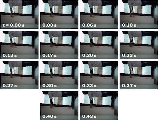
Figure 2. Frames from the video captured. The time 

interval between the images shown is 0.03 seconds.

     Now for the main image processing part. Using Scilab, we segmented the image using a patch of the ball from the image. Specifically we used Parametric segmentation to segment the image. Upon segmentation, we then binarized the image and computed for the centroid of the segmented portion. The centroid or geometric center [2] will give us the idea of the path taken by the ball as it was falling. We then combined each centroid extracted from the different frames to form one single image given by Figure 3.

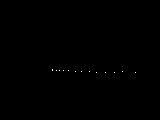
Figure 3. Path taken by the freely falling ball
represented by the centroid of each frame.

     From here, we identified the pixel position of each centroid. Noting that we can convert pixel position to actual distance using an image processing technique we learned from our very first activity, we then calculated for the actual distances for each pixel  position given in Figure 2. Plotting this with respect to the time we get.

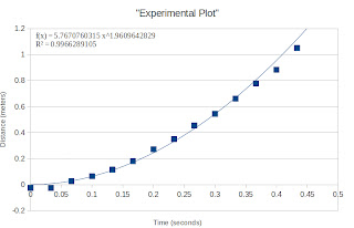
Figure 4. Distance versus  Time plot of a free falling ball. The 
distance was calculated through image processing means.

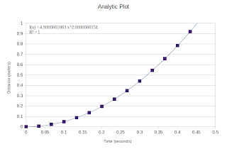
Figure 5.  Distance versus Time plot of a free falling ball. 

The distance was computed  using the equation for the 

falling distance of a free falling object.

     Note that the equation for falling distance is given by

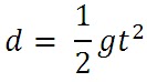
Equation 1. Falling distance equation, 

where d is the falling distance, g is the 

acceleration due to gravity and t is the

time.

     Therefore, upon fitting our plot with a power function we obtain g. The values obtained are given in Table 1.

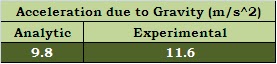
Table 1. Obtained Acceleration due to gravity (a) analytic 
computation, and (b)using image processing techniques.

     Note that the 1.8 m/s^2 difference can be explained by the "tilt" in the camera angle while capturing. This tilt causes a variation in our distance computations. Nevertheless, i'm so happy to have posted a blog (almost) on time again! :) Thank you Lord! :D And for that, I give myself a grade of 9/10. The one point deduction is partly due to the relatively large error of 18 %.  :)


God bless everyone! Have a great weekend ahead! :)

References:

[1] The zoetrope, retrieved  September 29, 2011, 
     http://www.exeter.ac.uk/bdc/young_bdc/animation/animation4.htm 
[2] Centroid, retrieved September 30, 2011, http://en.wikipedia.org/wiki/Centroid
[3] Soriano, M., A17 - Basic Video Processing, Applied Physics 186 Activity Manual, 2008