Back to the Basics

In order to master a subject one must know the basics - the ABC's and the 123's. Hence, in our second activity in our Applied Physics 186 class we did just that. We learned the basics of Scilab, a free software used for Numerical Computation. (Note: I'll be doing another blog regarding it's installation.)


Before anything else, the Scilab version I used in generating the images shown below was Scilab-4.1.2. I also installed the Scilab Image Processing (SIP) Toolbox to accomplish the activity.


Basically, our task was to generate different synthetic images. And, in generating these images the goal is for us to be familiar with the basics of Scilab. To help us get the job done, we were given an example to analyze. The code for a centered circle was given and is shown below.

Scilab code for a Centered Circle. 

Upon executing this in Scilab, the following image will be generated.

A Centered Circle. In optical systems this can be considered as a circular aperture

Here are the different synthetic images, with their corresponding Scilab code, that we were tasked to generate:

1. Centered Square Aperture

There are two ways in which I was able to generate this image. The first one is through the method below.

Scilab code for a centered square aperture (Method 1).

Centered Square Aperture (Method 1)

Here I made an nx x ny (for this specific case, 50 x 50) matrix of zeros. To achieve a centered square aperture, I "strategically" selected elements of the matrix. This works but it still seems primitive to me. Thus, the second  method that I used gives us a more elegant way of generating the image. 

Scilab code for centered square aperture (Method 2)

Centered Square Aperture (Method 2)

We basically start the same way we started for the first method. We create an nx x ny matrix of zeros. Now, it is in this next part where we "cut out" the square where this method becomes more advantageous. First, we locate the index of the center of the matrix (ie. A(i,j) where i and j are the indices) and from that we "select" a number of other matrix elements by adding and subtracting some value D to the indices of the element at the center of the matrix.

2. Sinusoid along the x-direction

Here I had to generate a matrix X which contained elements ranging from -1 to 1 and another matrix A which contained nx x ny zeros. I then applied the sine function to matrix X and equate it to matrix A as shown below. 

Scilab code for a sinusoid along the x-direction

Here is the resulting image,

Sinusoid along the x-direction (Corrugated Roof)

 3. Grating along the x-direction


For this part, I also have to different methods to generate the image. The first one requires "manual selection" which is quite primitive and messy in terms of the code used. The main idea is to select rows with an interval that you desire. These "cut out rows" in the matrix then contribute to the grating.

Scilab code for a grating along the x-direction (Method 1)

Grating along the x-direction (Method 1)

Since we desire a more practical method, here's one. To generate the grating, I just used the same concept in creating the corrugated roof. However, I used a function in Scilab that rounds up the values computed by the sine function, hence giving us a grating.

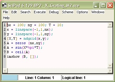Scilab code for a grating along the x-direction (Method 2)

Grating along the x-direction (Method 2)

4. Annulus

In generating an annulus we reuse some of the concepts in generating a centered circular aperture. The only difference here is that we will be adding two matrices to obtain the result we desire.

Scilab code for an Annulus

Annulus

5. Circular Aperture with Graded Transparency

Lastly, for a circular aperture with graded transparency, we will again use some of the concepts used in the centered circular aperture. The code is given below,

Scilab code for a circular aperture with graded transparency

Circular Aperture with Graded Transparency

For my self evaluation, i'd give myself a 12/10 for this activity. Special thanks goes to Jen-Jen Manuel for helping me understand Scilab better and for teaching me, giving me hints, and helping me figure out how to generate the images. Thanks to Arthur Galapon for helping me figure out how to generate the circular aperture with graded transparency.