Fourier Transform Model of Image Formation

What is Fourier transform?

     The Fourier transform belongs to the different classes of Linear transforms.[1] Linear transforms, in essence, "transforms" or "converts" information from one form to another. The Fourier transform, specifically, "transforms" a function with a dimension of G to a function with a dimension of 1/G. Moreover, given this function [say f(x,y)], it's Fourier transform is given by,

Equation 1. Equation for the Fourier transform of an image.

     In this activity, we will be using the Fast Fourier Transform to implement the Fourier Transform. Thankfully, Scilab has functions to implement this. They are fft() and fft2(). In addition, we will be using other Scilab functions that are new to us such as: fftshift(), abs(), conj(), and imcorrcoef().

     We now move on to the tasks we had to do. First off, we had to create a 128 x 128 image of a centered circle with white fill and black background. The image is then opened in Scilab and converted into grayscale.The Fast Fourier Transform for two dimensions was then applied. The intensity values were also computed and the following images were obtained.

Figure 1. (a) White centered circle made in paint. (b) fft2() 

of theimage in (a). (c) fftshift() applied to (b).

     I also did the same procedure for a white circle generated in Scilab. Here is the result:

Figure 2. White Circle generated through Scilab with the 
corresponding outputs of (a) fft2() and (b) fftshift()

     It can be seen that Figures 1 and 2 are almost identical if not for the difference in the radius of the white circle used. In addition to  these, if we apply fft2() again to the output of the fft2() of the grayscale image, we will obtain the white circle itself. Trying a different "object" in the image, we then used the letter "A" as shown below (this was generated through paint for obvious reasons).

Figure 3. (a) Our new "object" in the image. (b) the fft2() 

of a, (c) the fftshift() of (b).

What is a Convolution?

     You can imagine the convolution of two functions to be the smearing of one of the functions to the other. However mathematically, the convolution of two 2-dimensional functions, say, f and g, is said to be given by:

Equation 2. Convolution of two 2-dimensional functions f and g.

     A shorter way of representing the convolution of f and g is through the following manner.

Equation 3. Short-hand notation for 

the convolution of f and g

     Moreover, the convolution theorem states that,

Equation 4. Transform of the convolution h. Note that H, F 

and G are the transforms of h, f and g respectively.

   In this theorem, we see that the transform of the convolution h of two functions f and g is just the product of the transforms of f and g. And in the activity, we were tasked to do the following: (1) Create a 128 x 128 image with the letters VIP in it. I created this image using paint making sure the the letters occupy approximately 50% of the image. The font I used here is Arial. Here is the image,

Figure 4. Our object

     I then created another 128 x 128 image. A centered circle with white fill and black background. This image becomes our "aperture" of a circular lens. The next thing that we should do is to implement fft2() to Figure 5 and to  apply fftshift() to our aperture. Having done these, we multiply the two and get the inverse then display the modulus. Note that I varied the radius of the circle to observe the effect on the resulting image. The resulting images with the corresponding circles are seen in Figure 5.

Figure 5. Imaged "VIP" with corresponding lens aperture. The columns 

give a particular lens aperture with its corresponding imaged "VIP".

     The first observation that came to me when I saw these results (besides the fact that the resulting image is "upside down") is the quality of the resulting images. As one increases the radius of the circle the quality of the resulting image becomes better. Obviously, among all of these (including the object) the object has the greatest quality. 

What is Correlation?

     We now move on to correlation. In a nutshell, the correlation of two functions f and g gives the "extent" or degree of similarity of the said functions. [1] Mathematically, it is expressed as,

Equation 5.  Correlation of the two-dimensional functions f and g

     This can be written conveniently as,

Equation 6. Short-hand notation for the correlation
of two 2-dimensional functions f and g

     In addition, correlation is related to convolution in the following manner,

Equation 7. Relation of correlation to convolution

where the asterisk at f asks for the complex conjugate of f. Also, the transform of the correlation p is given by,

Equation 8. Transform P of the correlation p.  F and G are the transforms 

of  f and g respectively. F* is the complex conjugate of F

     Since the correlation gives us the degree of similarity of two functions, it is often used   in Template Matching. Template Matching is a technique used to detect parts of an image that match a particular template. [2] In the activity, we used an image with text to apply this technique. A template of a letter included in the text was then created. Note that the same font and font size for both the text in the image and the template was used. The results are shown below.

Figure 6. Application of correlation in an image with text. 

(a) template, (b) image with text. (c) resulting image.

     In Figure 6c we see the result. Note the positions of the letter "A" in (6b). If we compare it with Figure 6c, we see something interesting. Upon getting the transforms of (6a) and (6b) and applying it to Eq. (8) we get the transform P. And, taking it's inverse transform allows us to know the correlation p. Since the correlation gives us the degree of similarity between the template and the text in the image we know that the "brightest points" in (6c) has a high degree of similarity and therefore these letters match our template which is confirmed through our result. 

     

     Another thing that we did for correlation is edge detection. We used different patterns which were basically 3 X 3 matrices. The sum of all the elements in this matrix must be equal to zero. We then convolve this pattern with Figure 4. The result for each matrix is seen in Figure 7.

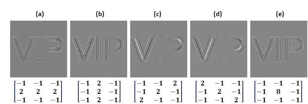Figure 7. Results for edge detection using different patterns of edges. 

(a)  horizontal pattern, (b) vertical pattern, (c) diagonal pattern going 

from left to right, (d) diagonal pattern going right to left,  and (e) spot

pattern.

     That ends our activity (Fourier Transform Model of Image Formation). It took me quite a long time to finish. However, I'm really amazed that I have finally finished it. Honestly, it's not that hard. It's actually quite simple and fun! And for that, i'd give myself a grade of 7 out of 10. All the images are of good quality and are with understandable captions. The 3 point deduction is due to the fact that I was late in posting my blog for this activity. Nevertheless, I had fun with this activity

     Thanks to Jen-Jen Manuel. Her post on this activity helped clarify some confusions with some of my results. 

All glory to God!

References:

[1] Soriano, M. A6 – Fourier Transform Model of Image Formation. Applied Physics 186 Manual. 2010.

[2] Template matching, retrieved September 22, 2011, http://en.wikipedia.org/wiki/Template_matching