A8 – Enhancement in the Frequency Domain

     If you haven't noticed, there have been previous posts here in my blog regarding Fourier Transforms, it's properties and the like. This is because knowing these tools (if you may) can help us in achieving "bigger" things. That having been said, in this activity we will utilize what we know so far of the fourier space and apply it to different situations. 

PART A: CONVOLUTION THEOREM

First off, let us look at the following 2D patterns:

Figure 1. (a) Two dots lying on the x-axis and symmetric about the y-axis.
(b) The modulus of the Fourier Transform of (a).

Figure 2. The first row is composed of images of two circles
of varying radius lying on the x-axis and symmetric about the
y-axis. The second row is the modulus of the Fourier Transform
of a respective pair of circles. 

      We have already seen Figure 1 in a previous blog. Now, instead of dots let us use circles of varying radius. From Figure 2, we observe that the FT modulus of our 2D pattern is given by "distorted" concentric circles. Moreover, as the radius of the circles increase the size of this interference pattern decreases. 

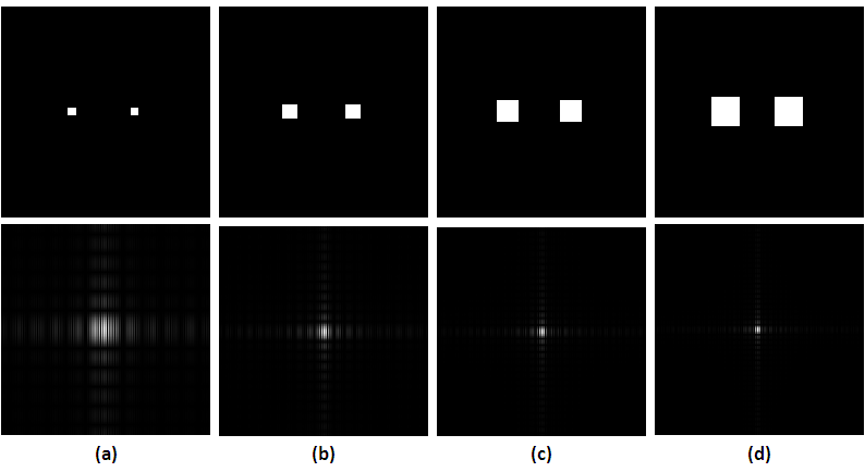Figure 3.The first row is composed of images of two squares
of varying side length lying on the x-axis and symmetric about the
y-axis. The second row is the modulus of the Fourier Transform of a respective pair of squares.  

     What if we replace the dots with squares instead of circles? In Figure 3, we see exactly that. In addition, given the respective fourier transform of each pair of squares we see that as the side length increases the  width of the distorted cross or plus sign  (interference pattern) decreases. 

Figure 4. The first row is composed of images of gaussians
of varying variance. The second row is the modulus of the
Fourier Transform of a respective gaussian pair. 

     Let us now try another 2D pattern - gaussians of varying variance. As seen in the Figure above (Figure 4), the interference pattern size decreases as the variance decreases. This trend is similar to the first two patterns.

     Another interesting thing that we will look at now is the convolution of two images. In Figure 5b we see the the result of the convolution of a vertical line (3x3) with the set of random points shown in 5a. What we see in 5b is the replication of the vertical line in every location where there is a random point. 

Figure 5. Convolution. (a) Random points. (b) Convolution
of a vertical line (3X3) to the random points of (a).

     To end this section, let us look at Figure 6. Our pattern are images with equally spaced dots that are on the x and y axis. Their corresponding FT modulus are also given in the figure.

Figure 6. The first column is composed of images of equally
Spaced dots lying on the x and y axis. The second row
is composed of the modulus of the FT of the images in the
first row. 

PART B: FINGERPRINTS: RIDGE ENHANCEMENT

Figure 7. Fingerprint (source)

     Given an image of a fingerprint, we can enhance the identifying marks or ridges in that fingerprint by masking unwanted frequency in the fourier  domain. We start with the following:

a. Take the Fourier transform of the image.

b. Design a filter for it.

c. Apply filter.

Figure 8. (a) FT modulus of Figure 7, (b) the filter I chose
to mask unwanted frequencies, and (c) Resulting image.

     Note that the output is not quite right. I would have to say that the error came from the choice of mask used.

PART C. LUNAR LANDING SCANNED PICTURES: LINE REMOVAL

     Applying masks can also be used in removing unwanted portions of an image. Here, we have an image where unwanted vertical marks is to be removed. I used the following mask in "filtering" the image.

Figure 9. Filter used in the image.

     Upon applying this, I was able to obtain the image in Figure 10b. I would have to say it looks pretty good.

Figure 10. (a) Image with unwanted vertical lines, (b) filtered image

PART D. CANVAS WEAVE MODELING AND REMOVAL

     Here is a similar case to the previous section. However, in this case we need to remove the weave marks instead of vertical lines. Shown in Figure 11 is 

Figure 11. Filter choice

Figure 12. (a) Image with weave marks. (b) filtered image.

     Unfortunately, it looks like the marks weren't removed. Once again, I strongly believe the error is in the choice of the filter.

Figure 13. (a) Inverted Filter. (b) FT modulus of (a) 

     Lastly, inverting the filter and taking it's FT modulus, we try to compare it with the weave pattern. Unfortunately, it does not resemble the weave pattern. However in my opinion it reminds me of the pattern (in an artistic manner) :D

     For this activity, I give myself a grade of 8 out of 10

     

     I'd like to thank the following people for their blogs: Jen Jen Manuel, Krista Nambatac, Tisza Trono, and James Pang. Because of their posts I am able to check my work and better understand the activity.

     God bless eveyone! :)