Properties of the 2D Fourier Transform

     In one of my previous blog posts, I have "introduced" the Fourier Transform. And now In this blog, we will be looking at its properties. This is important, because if we know some of its basic properties we will be able to, somehow, understand more complex situations involving Fourier Transforms.

     Below are some 2D patterns and their respective Fourier Transforms. I obtained the Fourier Transforms using Scilab.

Figure 1. 2D patterns with their respective Fourier Transform. 

A column corresponds for  a 2D Pattern - Fourier Transform 

pair. (a) Square, (b) Annulus, (c) Square Annulus, (d) Two slits 

along the x-axis and (e) 2 dots symmetric about the center.

     In  Figure 1 we see that given a certain 2D pattern, we obtain a distinct Fourier Transform. Note that in this particular work, the two slits  (Figure 1d) are symmetric about the center. Keeping these patterns in mind are important if we want to know more about Fourier Transforms. Moving on, below are 2D sinusoids along the x-direction. Just like in the first set of patterns, I took their Fourier Transforms. And as we see in Figure 2, as the frequency of the sinusoid increases, the distance between the two dots in the transforms of the sinusoids increases.

Figure 2. 2D sinusoids with their corresponding Fourier Transform.
A column represents a sinusoid-FT pair. (a) f =  4, (b) f =  8,
(c) f =  12, and (d) f =  16.

    Since digital images have no negative values, we add a bias to the sinusoid. Just like this,

Equarion 1. Sinusoid with bias A.

     Here A is the bias. And upon execution, we have the following:

Figure 3. Sinusoids with bias. (a) Constant 
bias of 10 and sinusoid frequency = 8, and (b) 
Sinusoidal bias of frequency 0.5 with same f = 8.

     Notice that in comparison to Figure 2b the FT of sinusoids with a bias has additional points. Specifically, for the constant bias, a dot at the center of the image can be seen, while two faint dots at the upper and lower portion of the images are present.  Given a non constant bias, two dots appear symettrical about the center in line with the y-axis. All of these dots (from the constant to non constant bias) obiously represent the FT for the respective biases.

     Let us now try to experiment with our 2D sinusoid. What if we rotate it? As seen in Figure 4 rotating the sinusoid also rotates its Fourier Transform. Once again, this fact is very helpful. Let us keep this in mind.

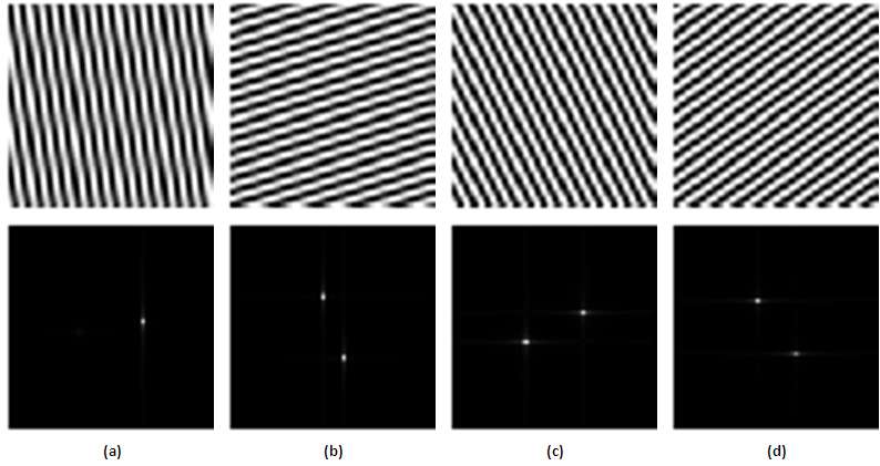Figure 4. Rotated Sinusoids with respective Fourier Transforms.
(a) theta = 30 ,  (b) theta = 60, (c) theta = 90, (d) theta = 120

     We now go to combinations of sinusoids. By combinations I mean product of sinusoids. And below, we see just that. Note that the observation that as the frequency of the sinusoid increases, the distance between the two dots also increase is also evident in Figure 5.

   

Figure 5. Combination of sinusoids in the X and Y together
with their respective Fourier Transforms. (a)  f =  4 , (b) f = 8.

Lastly, below are combinations of "regular" sinusoids and rotated sinusoids.

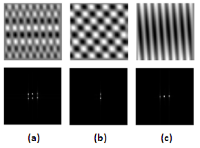Figure 6 Combinations of "regular" sinusoids and rotated
sinusoids. (a) X-Y-Rotated, (b)  X-Rotated, (c) Y-Rotated

For this activity, I would give myself a grade of 9 out of 10. 


I would like to acknowledge Jen-Jen Manuel and James Pang for their blogs. It helped me better understand this activity :)


God bless everyone! :D